Wireless Design · Antenna Theory, Pragmatically Applied
MIMO in WiFi Modules Explained: 2×2 vs 3×3 vs 4×4
TL;DR. Each MIMO antenna chain buys one spatially independent data stream — but streams beyond what the peer device and the propagation environment support are idle capacity. 2×2 fits most products and most clients (most phones are themselves 2×2). 3×3 is the sweet spot for sustained industrial links above roughly 600 Mbps. 4×4 buys real value only in high-density, many-client venues or carrier-style backhaul. Real TCP throughput is typically 55–70% of the PHY figure. Match chains to your actual client mix, sustained load, and power budget — not to the loudest number on the sheet.
A spec sheet will gladly tell you that more antennas means more speed. It will not tell you what those extra chains cost in power, board space, money, and cooling — or how often most deployments never need them. This guide is the honest, engineer-first answer to “which MIMO size do we actually need?”
- What the number next to × really means
- Why twice the streams is not twice the speed on paper
- The gap between PHY rate and real TCP throughput
- Six costs every extra chain carries
- A power and thermal budget worked example
- The antenna-isolation number you should ask for
- The tiered reality: what each size is really for
- The five mistakes that cost teams the most
- The client that crops your harvest
- MU-MIMO and OFDMA: when extra chains finally pay
- A decision matrix that avoids paying for idle capacity
- Putting a real chip next to each tier
- What an RF chain actually contains
- Form-factor and board tradeoffs you inherit
- Next-generation context: 802.11be
- The thermal footnote nobody reads in time
- Receivers, diversity, and the antennas you forget to buy
- Validating your choice before you commit
- A worked example: choosing for an outdoor gateway
- Glossary
What the number next to × really means
MIMO — Multiple-Input, Multiple-Output — is one of those acronyms everyone quotes and few people can explain cleanly. Stripped to its essence it is simple: a module equipped with several physical antennas can push several independent data streams (spatial streams) through the air at the same time on the same channel. The “2×2,” “3×3,” and “4×4” labels declare how many transmit-and-receive chains the radio contains — and therefore how many parallel data pipes it can keep open.
The first half of the label is the transmit chain count; the second is the receive chain count. Most practical modules are symmetric (2×2, 3×3, 4×4), but asymmetric examples exist, especially on the receive side where a chip may listen on more chains than it transmits. For the purposes of this guide — and for almost all module selection — symmetric ratios are the default you should plan around.
A spatial stream needs one chain on each end. Critically, the link is limited by the smaller of the two ends: a 4×4 access point talking to a 2×2 phone negotiates at most two streams. This single fact explains most of the confusion that follows, so it is worth stating plainly and repeating elsewhere in this piece.
Why twice the streams is not twice the speed on paper
Double the streams and you roughly double the raw link rate — provided channel width and modulation stay constant. Here is the theoretical (PHY) scaling across the three tiers, for the two most common channel widths in modern Wi-Fi:
| Configuration | Streams | Wi-Fi 5 · 80 MHz | Wi-Fi 6 · 80 MHz | Wi-Fi 6 · 160 MHz |
|---|---|---|---|---|
| 2×2 | 2 | 867 Mbps | 1.2 Gbps | 2.4 Gbps |
| 3×3 | 3 | 1.3 Gbps | 1.8 Gbps | 3.6 Gbps |
| 4×4 | 4 | 1.73 Gbps | 2.4 Gbps | 4.8 Gbps |
Two observations matter here. First, each doubling of streams does add real PHY capacity at a fixed channel width — that part of the marketing story is true. Second, the step from 2×2 to 3×3 adds one stream (a ~50% PHY jump at constant width), and 3×3 to 4×4 adds another (~33%). The relative lift shrinks as you climb, while the cost per added chain grows — the point of diminishing returns arrives sooner than the spec sheet suggests.
The gap between PHY rate and real TCP throughput
Treat PHY numbers as ceiling decoration, not achievable throughput. Real TCP throughput typically lands between 55% and 70% of PHY once protocol headers, contention, acknowledgements, and fading eat their share. Concretely:
- An 867 Mbps (2×2, Wi-Fi 5, 80 MHz) link usually behaves like a 450–600 Mbps connection.
- A 1.2 Gbps (2×2, Wi-Fi 6, 80 MHz) link more often delivers 700–850 Mbps in the field.
- A 4×4, 160 MHz PHY next to 4.8 Gbps is a lab-grade figure; sustained multi-client TCP is typically a fraction of it.
The practical takeaway: never size a link from its peak PHY. Size from a conservative TCP estimate for the client mix you actually expect, with a headroom margin on top.
Six costs every extra chain carries
The interesting part of MIMO choice is that it is not one dial. Adding a chain touches six things at once, and most of them are not “more speed”:
| Dimension | What it affects in practice | Why it matters |
|---|---|---|
| Throughput ceiling | Peak speed for a single-demand flow | Rarely the real constraint in most products |
| Concurrent clients | How many devices stay comfortable at once | The primary reason to go above 2×2 |
| Link margin | Each receive chain adds array gain (a few dB) | Stretches usable range at the edge of coverage |
| Noise / interference resistance | Spatial diversity and multipath handling | Helps in noisy, reflective environments |
| Power draw | Real current per RF chain | Directly caps battery life and thermal budget |
| BOM cost & area | Module, antennas, heatsink and layout | The reason 2×2 remains the default |
That is why the good design decision is usually the most careful one, not the biggest one. Every chain you add is borrowing against power, size, and budget you might spend more productively elsewhere — for example on a better antenna, a wider channel, or a faster uplink.
A power and thermal budget worked example
To make the tradeoff concrete rather than abstract, run a simplified power accounting yourself. The exact numbers depend on chip and TX power, but the shape of the calculation is what matters:
3×3 aggregate draw: ~4–6.5 W (one extra chain + PA)
4×4 aggregate draw: ~5.5–9 W, >10 W with high-TX PA
Budget guide: pick a tier whose worst-case draw your rail and chassis tolerate all afternoon
Now imagine a PoE+ powered outdoor AP. PoE+ (IEEE 802.3at) offers up to ~30 W at the PSE, less after cable and injector losses. A 2×2 radio leaves huge headroom; a 4×4 at high TX power starts to crowd the budget once you add the baseband, any peripherals, and the loss of delivering power over the cable. The same principle applies to battery-powered IoT, where the difference between a 2×2 and a 4×4 can be the difference between months and weeks of runtime.
There is no universal cap — the right call is a function of your rail, your enclosure, and your duty cycle. But the discipline of writing down the worst-case power budget before choosing the tier is common to every good design.
The antenna-isolation number you should ask for
Because all chains radiate on the same frequencies, keeping them from interfering with each other is the difference between genuine MIMO and an expensive nominal MIMO. As a rule of thumb:
- Aim for roughly 20–30 dB isolation between any two chain antennas for useful MIMO operation.
- In a compact form factor, achieving that isolation is the hard part — it is why larger cards with more spacing often outperform denser module designs at the same chain count.
- Request the isolation figure from the vendor alongside the throughput table; a datasheet that quotes streams but not isolation is telling you only half the story.
This is fundamentally a board-and-antenna engineering question. The RF performance and layout guide walks through antenna termination, matching, and the isolation realities in detail.
The tiered reality: what each size is really for
Here is the honest characterisation of each tier, grounded in typical reference designs and the real loads they serve.
These are ranges, not absolutes — exact current and throughput depend on the specific chip, firmware, channel width, and how well your board executes the RF design. The relative ordering, however, holds across vendors.
The five mistakes that cost teams the most
Most MIMO mistakes are not about picking the wrong tier — they are thinking about the tier the wrong way. Here are the five that routinely cost real money:
- Sizing from peak PHY. Quoting the 4.8 Gbps line on the datasheet as if it were achievable TCP. It is not; use 55–70% of PHY and size from sustained load.
- Ignoring the client mix. Buying 4×4 for a fleet of 2×2 phones. The extra streams only help with true simultaneous multi-flow load.
- Forgetting the antennas. Picking a 4×4 module in a chassis that cannot host four well-isolated antennas, so the concurrency capacity never materialises.
- Neglecting the thermal envelope. Installing the extra chains in a sealed box with no airflow, then watching MCS collapse (and throughput follow) on a warm afternoon.
- Confusing streams with speed. Assuming a phone gets a four-stream link because the AP is 4×4. The link is limited by the client’s chain count, not the AP’s.
All five are avoidable with the same habit this whole guide drives at: name the real workload, measure the 55–70% TCP reality, check the antennas and the heat before you buy — then and only then choose the tier.
The client that crops your harvest
One myth deserves a direct rebuttal: buying a 4×4 module does not give a phone a four-stream connection. Most clients — smartphones, sensors, and laptops — are themselves 1×1 or 2×2. A 4×4 AP physically cannot pour four streams into a two-stream client; the extra streams are only usable by other simultaneous clients via multi-user techniques, or as buffered capacity for parallel users.
This reframes the decision. If your real fleet is mostly 2×2 clients, a 4×4 AP buys concurrency and headroom, not faster single-client speed. Before paying for four chains, ask what fraction of your clients can actually use them simultaneously and whether your traffic is dense enough to need parallel streams at once.
MU-MIMO and OFDMA: when extra chains finally pay
The reason to go above 2×2 lives in the multi-user features rather than the headline rate:
- MU-MIMO lets a radio transmit downlink to several single-stream clients at the same time on different spatial streams. Four chains literally enable serving four different devices in one burst, which is how 4×4 helps high-density areas.
- OFDMA (in Wi-Fi 6 and later) is a separate mechanism that subdivides the frequency resource, letting an AP carry many small clients in parallel regardless of MIMO count. It raises efficiency in the many-small-clients case even on a 2×2 radio.
Practical guidance: if your workload is one or two heavy flows, more chains barely help. If it is dozens of light clients, OFDMA may matter more than a third or fourth MIMO chain. If it is several simultaneous heavy streams, MU-MIMO and more chains genuinely pay. Match the mechanism to the traffic shape, not to a reflex for the top tier.
A decision matrix that avoids paying for idle capacity
| Your real constraint | Look at | Likely size |
|---|---|---|
| Per-client link speed on 80 MHz | Typical TCP for your client mix | 2×2 is usually enough |
| Sustained industrial link > ~600 Mbps | Mid-tier aggregate TCP throughput | 3×3 often the best value |
| High density / many concurrent clients | MU-MIMO concurrency + OFDMA | 4×4 |
| Tight power or battery budget | Active + idle draw in sealed enclosure | 2×2, with power-save |
| Edge-of-range coverage for a few clients | Receive chain array gain | Often simpler than a third chain |
Notice the pattern: the smallest configuration that meets your throughput ceiling, client count, and power budget is nearly always the right engineering answer. Streams you never use still draw current, still cost money, and still need cooling.
Putting a real chip next to each tier
Concrete examples help the decision stop being abstract:
- The Qualcomm QCN9074 sits at the top — a 4×4, Wi-Fi 6 radio doing up to ~2.4 Gbps at 80 MHz, aimed at enterprise APs and carrier CPE. It is the reference point when the capacity play is legitimate.
- The QCA9880 is the classic 3×3, Wi-Fi 5 chip — the price-to-performance favourite for industrial bridges and mid-range APs that need more than a single pair of streams.
- On the value end, the QCA9882 or a 2×2 Wi-Fi 6/5 part fits cost-optimised gateways where unit BOM, power, or board area is the deciding constraint.
For a deeper look at any single tier, the QCN9074 deep-dive covers the 4×4 case, and the generation-selection guide situates these choices alongside Wi-Fi generation.
The thermal footnote nobody reads in time
Nobody enjoys discovering this late: a high-stream module inside a sealed housing is a heat source. A 4×4 under a heavy stream can approach 5–9 W of draw, and at higher TX power that climbs past ~10 W with high power amplifiers. If your enclosure has no active cooling, the extra chains you bought for peak throughput may be throttled back by the very thermal envelope you installed them in. Before committing to the four-chain board, check its thermal budget against your worst-case ambient temperature and your enclosure.
This is a recurring theme across Wi-Fi module design. The industrial temperature guide and the outdoor metal-enclosure guide both go deeper on the interaction between heat, derating, and throughput.
Receivers, diversity, and the antennas you forget to buy
A module is only as good as the antennas it is paired with. Two chains are useful even when you only need one stream, because the second receive chain provides receiver diversity — the radio can pick the stronger of two signals in a fading environment, which measurably helps range and reliability. That is one honest case where a second chain earns its keep without any throughput story.
But each chain also needs a physically separate antenna with adequate isolation, or the whole MIMO benefit erodes into self-interference. Plan the antenna count, spacing, and cable loss into your BOM before you celebrate the module’s stream count. The cleanest way to see this is the board and RF performance guide, which treats layout, matching, and antenna termination as inseparable from the radio.
What an RF chain actually contains
Behind the neat “2×2” label is real hardware on the board, and it explains neatly why every added chain is expensive. Each transmit chain needs a baseband DAC output, an up-converter, a power amplifier, a band-pass filter, an antenna switch, and the antenna itself. Each receive chain needs its own low-noise amplifier, down-converter, and ADC. When you go from two chains to four, you are not merely doubling a number — you are nearly doubling a bill of materials and a power budget and a thermal load:
Per RX chain: antenna → switch → LNA → down-convert → ADC → baseband
Consequence: 4×4 roughly doubles parts, current, and board area vs 2×2
This is the mechanical reason a 2×2 module can ship in a compact, low-power card while a 4×4 part needs a bigger footprint, a better thermal path, and a supplier with the RF integration skill to keep all four chains isolated from one another. When a vendor sells a “cheap” 4×4 module, scrutinise how they handled isolation and power — corners get cut exactly where they are hardest to see.
Form-factor and board tradeoffs you inherit
The chain count leaks into your mechanical design whether you plan for it or not. Two chains need two antennas with suggested isolation of roughly 20–30 dB between them for good MIMO performance; four chains need four antennas with the same per-pair isolation on a board that did not necessarily grow. In a compact gateway or an IoT module the antenna budget frequently becomes the real constraint long before the radio does.
The practical routing is straightforward but worth stating: the faster the MIMO tier, the more of your design effort and cost goes to antenna placement, cable routing, and RF layout, and the less it looks like a software decision at all. If your mechanical envelope cannot host well-isolated antennas, the 4×4 capability on the datasheet is theoretical. This is covered in concrete, layout-level detail in the RF performance and board-layout guide.
Module form factor also tracks the tier loosely: 2×2 Wi-Fi parts commonly ship on compact M.2 or Mini-PCIe cards and small LGA modules, while 3×3 and 4×4 parts appear on larger cards and developer boards with more RF real estate. Selecting a chain count is therefore also selecting a class of module form factor — a constraint worth confirming with the vendor early, because changing it late is a redesign, not a swap.
Next-generation context: 802.11be and more width, not more of the same
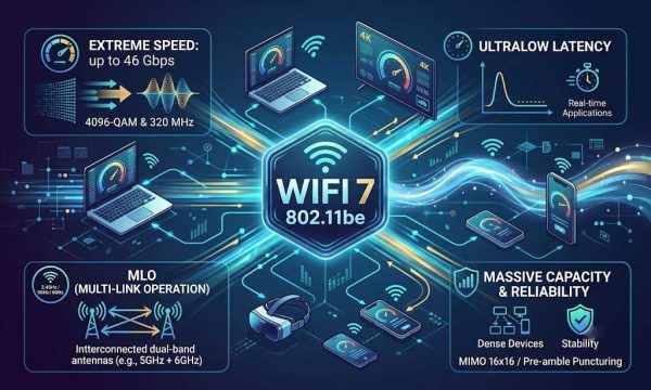
It is worth placing MIMO in the trajectory of the standard, because the next generation changes the emphasis. Wi-Fi 7 (802.11be) keeps stream counts in familiar territory — 2×2, 4×4 — but its headline speed gains come chiefly from 320 MHz channels, 4096-QAM modulation, and multi-link operation (MLO), rather than from climbing to a higher MIMO tier. That means the “more streams or bust” instinct is even less applicable for Wi-Fi 7 products.
For full detail see the dedicated Wi-Fi 7 speed and features guide. The MIMO message remains: match chains to clients and load, and let wider channels and smarter scheduling carry the next-generation speed story.
| Generation | Primary speed levers | Typical stream counts |
|---|---|---|
| Wi-Fi 5 (ac) | 80/160 MHz + up to 4×4 | 2×2 – 4×4 |
| Wi-Fi 6/6E (ax) | OFDMA + MU-MIMO + 160 MHz | 2×2 – 4×4 |
| Wi-Fi 7 (be) | 320 MHz + 4096-QAM + MLO | 2×2 – 4×4 (often stays low) |
Validating your choice before you commit
An informed paper decision is still worth a real-field confirmation. A short validation plan de-risks the module choice in a few focused steps:
- Model your TCP ceiling. Estimate 55–70% of PHY for your widest supported channel width and client type.
- Enumerate the real client mix. Count stream capabilities, not just device count — most phones are 2×2.
- Test at the edge. Measure TCP at the coverage boundary, where modulation collapses and margins shrink most.
- Stress concurrency. Drive 20–120 synthetic clients and watch aggregate throughput and per-client latency under MU-MIMO and OFDMA.
- Run the thermal test. Seal the enclosure, run max sustained load, and watch for MCS collapse or throttle events on hot days.
Skip the thermal test and the concurrency test on a dense or outdoor design and you will meet exactly the class of failure documented in our 60-client edge-gateway field story — where the radio was never the constraint and the pipeline was. The same discipline applies here: size and validate from real load, not peak spec.
A worked example: choosing for an outdoor gateway
To tie the whole piece together, consider a concrete decision: a pole-mounted gateway serving public Wi-Fi to tens of passing visitors and a handful of sustained camera streams. Working through the constraints systematically:
- Client mix. Public visitors are mostly 2×2 phones; cameras are often 1×1 uplink devices. Very few clients exceed two streams.
- Traffic shape. Many light, short-lived connections for visitors plus a few sustained uplink video flows — a classic OFDMA-plus-MU-MIMO mix, not a single heavy stream.
- Power and thermal. Sealed pole chassis with modest enclosure area and a single PoE+ line. There is little room to dissipate a high-watt multichain radio at 4×4.
- Conclusion. A 2×2 Wi-Fi 6 radio comfortably satisfies the 20–35 concurrent visitor case while the OFDMA mechanism handles the many-small-flows efficiently, and the thermal power fits the PoE+ rail. A 4×4 radio would add cost and heat with little benefit — exactly the conclusion reached in practice in our 60-device gateway field story.
That same reasoning — name the clients, name the traffic shape, name the power budget, then pick the smallest tier that satisfies all three — generalises to almost every module selection. It is the difference between a MIMO decision and a MIMO guess.
Frequently asked questions
What does 2×2, 3×3 and 4×4 MIMO actually mean?
The label declares how many transmit-and-receive chains the radio contains — the first number is transmit chains, the second receive. Each chain can push one independent spatial stream on the same channel, so a 4×4 radio holds up to four parallel data pipes. Most practical modules are symmetric (2×2, 3×3, 4×4).
Does a 4×4 access point make my phone faster?
No. The link is limited by the smaller of the two ends: a 4×4 AP talking to a 2×2 phone negotiates at most two streams. Most clients are 1×1 or 2×2. A 4×4 AP buys concurrency and headroom for simultaneous clients, not faster single-client speed.
What is the real throughput of a MIMO link?
Real TCP throughput typically lands between 55% and 70% of the PHY rate once headers, contention, acknowledgements and fading take their share. An 867 Mbps (2×2 Wi-Fi 5, 80 MHz) link usually behaves like a 450–600 Mbps connection; a 1.2 Gbps (2×2 Wi-Fi 6) link delivers roughly 700–850 Mbps. Never size a link from its peak PHY.
Which MIMO size should I choose?
2×2 is the default workhorse for IoT gateways and small APs (20–35 concurrent clients). 3×3 is the industrial-link sweet spot for sustained traffic above ~600 Mbps. 4×4 is a capacity play for high-density venues, enterprise APs or carrier backhaul (80–120+ clients). Choose the smallest tier that meets your throughput, client count and power budget — unused streams still draw current.
Why does MIMO cost more than just speed?
Every added chain touches six things at once: throughput ceiling, concurrent-client capacity, link margin, noise resistance, power draw, and BOM cost and area. A 4×4 radio can draw around 5.5–9 W (over 10 W with high-TX power amplifiers) versus roughly 2.5–4.5 W for a 2×2, which stresses battery life, thermal envelopes and PoE budgets.
Glossary
- MIMO
- — Multiple-Input, Multiple-Output; using several antennas and chains to carry independent spatial streams.
- Spatial stream
- — one independent data pipe carved out of the radio’s antennas; the multiplier in the PHY rate formula.
- Chain (TX/RX)
- — a complete transmit or receive RF path; the number of chains sets the MIMO count.
- MU-MIMO
- — Multi-User MIMO; transmitting to several single-stream clients on different chains simultaneously.
- OFDMA
- — Orthogonal Frequency Division Multiple Access; subdividing the channel to carry many small clients in parallel.
- PHY rate
- — the theoretical physical-layer data rate before protocol overhead and interference.
- Receiver diversity
- — using a second receive chain to pick the stronger signal, improving range without adding a stream.
Related Reading
- Choosing a WiFi module generation
- A 4×4 Wi-Fi 6E radio for dense rooms
- Wi-Fi 7, MLO and multi-link
- Wi-Fi 5 product decisions in context
- Board layout and RF performance
- A gateway running 60 clients at once
Sources & further reading
- IEEE, 802.11 MIMO / spatial streams and multi-user transmission — IEEE 802.11
- Wi-Fi Alliance, MIMO and multi-user MIMO in Wi-Fi 5 / Wi-Fi 6 — wi-fi.org
- Qualcomm, QCN9074 802.11ax 4×4 radio — qualcomm.com
- Antenna theory reference — antenna-theory.com
Figures above are directional reference values from typical reference designs and public documentation; exact rates and current draw depend on the chipset, firmware, channel width, modulation, and antenna execution on your specific board. Validate throughput and thermal behaviour on your own hardware before committing to a MIMO tier.