Industrial Mesh Networks and Dedicated Roaming Clients: Coverage Gaps, Deployment Models and Selection Guide
Key Overview
Who this article is for: engineering leads, procurement managers and technical selection teams building wireless networks for factories, mines and warehouses — and non-technical readers who want a quick answer to “if Mesh already supports roaming, why buy a separate roaming device?”
Core question: How do Mesh self-organizing networks and dedicated roaming clients actually relate? Why is a separate roaming client still needed once Mesh is in place? How should the two be combined to be both cost-effective and reliable?
Key conclusion: A Mesh network is the infrastructure layer — a self-healing wireless coverage fabric for sites where cabling is impractical. A dedicated roaming client is the deterministic guarantee at the endpoint — it keeps robots and AGVs communicating while they move. The two are complementary, not interchangeable: infrastructure and endpoint. If the application tolerates a brief pause at handover (inspection video, for example), built-in Mesh roaming is sufficient. If a pause means an AGV drifts off its path, a line stops, or a remote-control command is lost, dedicated hardware with Make-before-break handover logic is mandatory.
1. Core Concepts: Mesh Self-Organizing Networks and Roaming Clients
1.1 Mesh Self-Organizing Network (the Infrastructure Layer)
Picture a mine shaft or machine hall where pulling cable is not an option, and you need wireless coverage across the entire site. The conventional approach is to run a cable to an AP at every location — expensive, slow to install, and a single cut cable takes out that whole area.
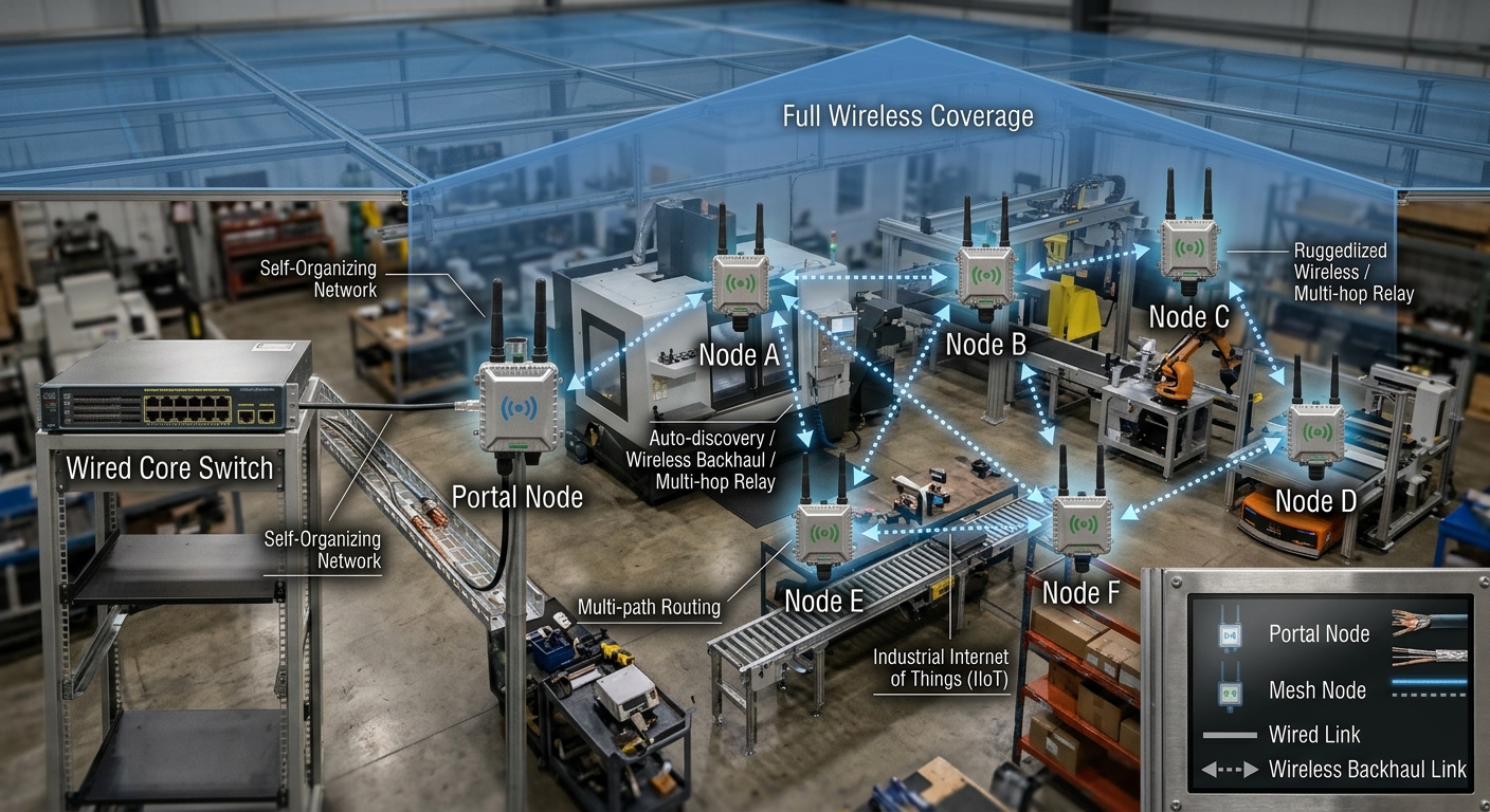
Mesh networking exists to solve exactly this problem. It is a decentralized topology: multiple Mesh nodes are distributed across key positions in the work area and interconnect automatically over the air, forming the network on their own.
1.1.1 How a Mesh Network Comes Up: Three Steps
- Step 1 — Power up and place the nodes. At least one Mesh node is cabled and configured as the Portal node — the gateway that bridges the wireless Mesh to the plant’s wired backbone. The remaining nodes need only power; set them to Client mode and position them at the planned locations (one every 100–150 m).
- Step 2 — Automatic discovery and association. On power-up, every node scans for neighbouring Mesh signals, authenticates using the pre-provisioned SSID and passphrase, and automatically establishes wireless backhaul links to form the mesh topology. This typically takes only tens of seconds.
- Step 3 — Self-healing and path selection. Each node maintains links to multiple neighbours. When a link degrades or a node loses power, the protocol reroutes traffic automatically. Nodes can be added, removed or relocated on site at any time, and the network converges on a new optimum topology by itself.
1.1.2 Mesh Network Architecture
1.1.3 Mesh Topology Evolution
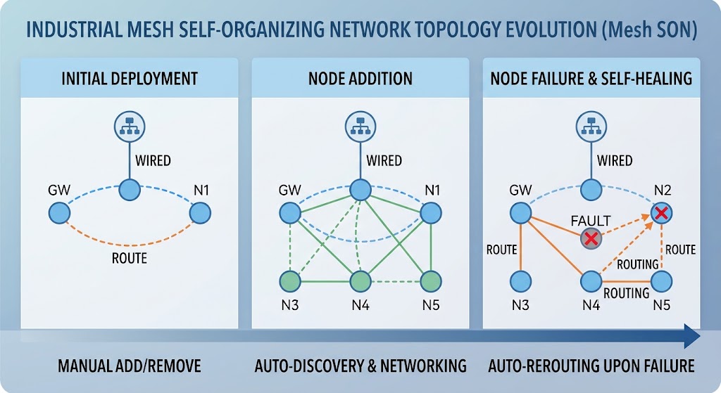
- Decentralized and self-healing: there is no single central base station. If any node fails, the network finds an alternative path — ideal for underground workings and mining areas where the environment is harsh, cabling is difficult and equipment is easily damaged.
- Multi-hop relay for coverage extension: nodes relay traffic over wireless backhaul. Deploying one node roughly every 100 m delivers site-wide coverage without additional cabling.
- Baseline roaming support: some industrial Mesh products support 802.11k/v/r or vendor-specific fast roaming to assist client handovers.
1.2 Roaming Client (the Endpoint Layer)
A roaming client is an industrial wireless module installed on mobile equipment — AGV robots, autonomous mining trucks, RGV shuttle carts. Its job is to:
1.2.1 How a Roaming Client Works: From Handover to Seamless Roaming
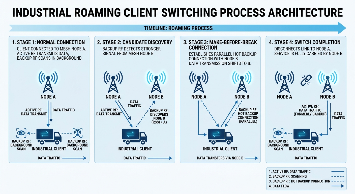
- Background scanning, always ready. The client does not wait for the link to drop. While the current link carries traffic normally, a secondary radio continuously scans the signal strength of surrounding Mesh nodes. The scan is independent and does not affect ongoing data transfer.
- Threshold-triggered, client-initiated handover. When a candidate node is stronger than the current one, or the current link falls below a configured threshold (for example -70 dBm), the client initiates the handover immediately. The decision is made autonomously on the client side, without waiting for a network-side command.
- Fast handover, no data loss. A dedicated roaming client uses Make-before-break logic: while the current link is still healthy, it has already established a connection to the new Mesh node over the secondary radio, and traffic is switched seamlessly from the hot-standby path. There is no break window, and latency can be held below 10 ms.
1.2.2 Roaming Client Handover Flow
- Carries robot control and sensor data back over the wireless network
- Handles AP-to-AP handovers automatically as the robot moves from point A to point B across different Mesh node coverage areas
- Provides industrial-grade protection (wide temperature range, vibration resistance, DIN-rail or vehicle mounting) and lets the robot’s wired equipment — PLCs, industrial PCs, sensors — join the wireless network
2. Why Built-in Mesh Roaming Is Not Enough
Mesh already includes roaming, so it sounds like every scenario is covered. Yet many industrial projects still buy dedicated roaming clients on top. The answer lies in the nature of the Mesh architecture itself.
2.1 The Decision Still Rests with the Client
Mesh nodes can supply a neighbour AP list and handover suggestions to the client via 802.11k/v, but the client executes the handover.
Think of Mesh as a diligent navigation system repeatedly telling you to take the next exit — but if you (the client’s roaming algorithm) ignore it, or your decision logic is off, and you insist on sticking to the old node whose signal has already degraded, the navigation system has no way to force the turn.
2.2 The Cost of Passive Reconnection
Conventional mesh networks designed around static nodes typically rely on passive reconnection after the link drops: disconnect, rescan channels, re-authenticate, re-associate. The whole sequence can take hundreds of milliseconds — a break-then-connect handover.
Even with 802.11r fast roaming enabled, the mechanism is still break-before-make: the current link is torn down first, then authentication is restored quickly on the new AP. For millisecond-sensitive traffic such as AGV control commands or remote mining-truck operation, that break is the risk window.
3. What Dedicated Roaming Hardware Does Better: Uninterrupted Handover, Guaranteed Latency
3.1 Radio Redundancy: Dual/Multi-Radio Removes the Scan-vs-Transmit Conflict
A general-purpose industrial AP uses the same radio for data and background scanning, so scanning steals airtime from traffic — like trying to take a phone call and find your way at the same time, with both suffering.
Dedicated roaming devices use a dual-radio or even quad-radio architecture: one radio maintains the active session, while another continuously and independently scans and evaluates candidate links. Scanning consumes no service bandwidth — two people dividing the work, one on the call and one navigating.
3.2 Handover Logic: Make-before-break Replaces Break-before-make
This is the most fundamental difference between dedicated industrial solutions and generic Mesh roaming. Dedicated solutions generally use Make-before-break logic:
- While the current link is still healthy, the mobile node has already established parallel connections to multiple candidate base stations over the secondary radio
- Traffic is pre-transmitted or held in hot standby across those paths
- When the original link degrades, the traffic stream switches directly to the already-prepared path — there is no moment of disconnection
The result: failover time can be held below 10 ms, far better than the hundreds of milliseconds typical of 802.11r-based fast roaming.
3.3 Deterministic Industrial Metrics
Dedicated solutions commit to verifiable figures rather than “best effort”:
| Metric | Generic Mesh roaming | Dedicated industrial roaming |
|---|---|---|
| Handover latency | Tens to hundreds of ms, highly variable | <10 ms – 50 ms, deterministic |
| Packet loss | Possible loss at the handover instant | Zero loss or <0.05% |
| Supported mobility | Low speed | Stable link at 80 km/h |
| Typical applications | Inspection data, non-real-time monitoring | AGV/AMR control, remote mining-truck operation, high-speed production lines |
3.4 Dedicated Mobile Mode Handles Cross-Channel and Topology Changes
When a mobile node crosses subnet or channel boundaries, generic Mesh nodes tend to stay locked to the current channel and lack initiative — often dropping the link outright. Dedicated mobile mode instead:
- Performs active cross-channel scanning and route rebuilds
- Optimizes neighbour scan intervals and route convergence for high-speed mobility
- Suppresses retransmissions caused by multipath fading
4. Selection Comparison: The Differences at a Glance
4.1 Built-in Industrial Mesh Roaming vs Dedicated Industrial Roaming Hardware
| Dimension | Built-in industrial Mesh roaming | Dedicated industrial roaming device/mode |
|---|---|---|
| Handover logic | Client-decided, break-then-reconnect | Network/hardware-driven, Make-before-break |
| Radio foundation | Single/dual radio, scanning shares airtime with traffic | Dual/multi-radio, scanning physically isolated from traffic |
| Handover latency | Tens to hundreds of ms, highly variable | <10 ms – 50 ms, deterministic |
| Packet loss | Possible loss at the handover instant | Zero loss or very low loss (<0.05%) |
| Mobility support | Low to moderate speed | Stable link at 80 km/h |
| Typical industrial workloads | Inspection data backhaul, non-real-time monitoring | AGV/AMR control, remote mining-truck operation, high-speed production lines |
| Typical vendor/technology | Standard 802.11k/v/r | Vendor-specific fast roaming (e.g. proprietary zero-switch protocol) |
| Cost | Included with the Mesh equipment, no extra spend | Requires separate industrial clients, higher unit cost |
4.2 The Decision in One Sentence
Three reasons behind that decision:
(1) You Do Not Control Built-in Mesh Roaming
Mesh nodes can give the client a neighbour AP list and handover suggestions, but whether and when the client acts depends entirely on its own roaming algorithm. Different vendors’ clients — even different batches of NICs from the same vendor — can behave differently. For inspection video or non-real-time monitoring, where an occasional stutter is acceptable, that does not matter. For AGV control or remote mining-truck operation, where a single break is an incident, it is a time bomb: you cannot predict when the client will stick to a weak-signal node and refuse to move.
(2) Dedicated Roaming Hardware Eliminates the Uncertainty by Design
Dedicated devices use a dual-radio architecture to physically isolate scanning from traffic, and Make-before-break logic to turn “disconnect first and hope” into “build the new link, then switch”. Both design choices bypass client-side unpredictability at the hardware level, cutting handover latency from hundreds of milliseconds to under 10 ms and turning packet loss from “possible” into “committed”. That determinism is not an optimization — it is inherent in the architecture.
(3) The Cost Premium Must Match the Business Value
Built-in Mesh roaming comes with the Mesh equipment — buy a Mesh node and you have it, at no extra cost. Dedicated roaming clients are purchased separately and cost considerably more per unit. Selection therefore comes down to a risk calculation: is the application worth paying extra for determinism? If the loss from a single failed handover exceeds the cost of the client, the answer is yes.
4.3 YN700B Mesh Board vs YN300B Seamless Roaming Client
To make the selection concrete, the table below compares measured specifications of two boards from the same vendor — the Mesh backbone node on the left, the dedicated roaming client installed on the AGV on the right. Used together, roaming protocol and RF parameters are fully aligned: the classic same-vendor pairing.
| Parameter | YN700B Mesh board (backbone side) | YN300B seamless roaming client (endpoint side) |
|---|---|---|
| Chipset | Qualcomm AR9344, MIPS 74Kc, 560 MHz | Qualcomm platform (model not disclosed) |
| Operating band | 5.8 GHz only (5.180–5.825 GHz) | 5.8 GHz (single-band design, roaming capable) |
| Transmit power | 30 dBm (1 W), factory-set per regional regulations | 30 dBm (1 W), factory-set per regional regulations |
| Receiver sensitivity | -97 dBm @ 20 MHz | -97 dBm @ 20 MHz |
| Antenna technology | 2×2 MIMO | 2×2 MIMO |
| Actual wireless throughput | Up to 96 Mbps | Up to 96 Mbps |
| Channel bandwidth | 5/10/20/40 MHz, configurable | 5/10/20/40 MHz, configurable |
| Range (elevated, clear line of sight) | 3–8 km | 3–8 km |
| Mesh scale | ≥50 nodes, ≥10 relay hops | Joins the Mesh network as an endpoint |
| Role | Mesh backbone node / relay / portal | Roaming client / mobile endpoint access |
| RJ45 ports | 10/100M × 2 | 1000M × 2 (dual Gigabit) |
| GPIO | 5 | 12 |
| Power input | 12–48 V DC / PoE | 7–48 V DC / 15–48 V PoE |
| Average power consumption | 15 W | 10 W |
| Operating temperature | -40 °C to +65 °C | -40 °C to +65 °C |
| Software | Bootloader with recovery + web configuration | Bootloader with recovery + web configuration |
| Roaming capability | Baseline roaming built into the Mesh stack | Single-band seamless roaming (dedicated mobile mode) |
| Installation | Fixed on workshop walls / columns / tunnel walls | Vehicle-mounted or embedded on AGVs, mining trucks and other mobile platforms |
Key observation: in a same-vendor pairing, the Mesh backbone node and the roaming client share identical RF parameters (-97 dBm sensitivity, 2×2 MIMO, 30 dBm transmit power). This combination of aligned RF and a common protocol stack is where roaming performance is easiest to maximize — handover suggestions from the AP side are recognized and acted on by the client without ambiguity.
4.4 Transmit Power and Regional Regulatory Limits: 30 dBm Is a Compliance Ceiling, Not a Performance Limit
First, Separate Two Concepts: Conducted Power vs EIRP
Many readers confuse “30 dBm” and “36 dBm” in datasheets. They are two different reference points:
- Conducted power: the power delivered at the radio port, excluding antenna gain. The “30 dBm” in a datasheet usually refers to this.
- Equivalent isotropically radiated power (EIRP): conducted power plus antenna gain. Radio regulations typically limit EIRP, because that is what actually represents the energy radiated into the air.
The relationship is simple: EIRP = conducted power + antenna gain. For example, 30 dBm conducted with a 6 dBi antenna gives 36 dBm EIRP. The same device with a higher-gain antenna may therefore exceed local limits — a point easily overlooked during selection and customs clearance.
5.8 GHz Power Limits in Major Markets
| Region / certification | Band | EIRP limit | Conducted power equivalent with 6 dBi antenna | Notes |
|---|---|---|---|---|
| China (MIIT / SRRC) | 5725–5850 MHz | ≤ 33 dBm (approx. 2 W) | approx. 27 dBm | Antenna gain ≤ 12 dBi; domestic firmware locks power to this limit |
| China (2.4 GHz, for reference) | 2400–2483.5 MHz | ≤ 20 dBm (100 mW) | approx. 14 dBm | 2.4 GHz power is inherently constrained — one reason industrial deployments favour 5.8 GHz |
| United States (FCC Part 15.247) | 5725–5850 MHz | ≤ 36 dBm (4 W) | approx. 30 dBm | Full 30 dBm conducted power is usable with antennas up to 6 dBi; a relatively permissive limit |
| European Union (ETSI EN 301 893) | 5725–5875 MHz | ≤ 30 dBm (1 W) | approx. 24 dBm | More conservative than China or the US; CE marking required |
| Japan (MIC / TELEC) | 5.8 GHz band | ≤ 30 dBm | approx. 24 dBm | TELEC (technical conformity) certification required |
Note: the table shows typical limit ranges. The latest local regulations and certification body requirements take precedence; specific limits may also vary with antenna gain and channel bandwidth. The “conducted power equivalent” column assumes a 6 dBi antenna and is for intuitive comparison only.
Why Transmit Power Can Be Customized at the Factory
The RF chipsets in the YN700B / YN300B support software power control, so different power levels can be configured at the factory according to the destination market:
- Domestic sales: firmware locks power to EIRP ≤ 33 dBm, so the unit with its supplied antenna passes SRRC type approval directly
- Export to the US: can be opened up to 30 dBm conducted with a 6 dBi antenna (36 dBm EIRP), meeting FCC Part 15.247
- Export to the EU: factory-set to EIRP ≤ 30 dBm, meeting ETSI EN 301 893 and CE requirements
- Special projects (e.g. private networks at mines or ports): band and power can be customized to customer specification, in line with the local radio authority’s spectrum licence
This is a key difference between industrial-grade equipment and consumer routers — consumer products have fixed power, while industrial equipment must be configurable per project and per region, otherwise a single model could never be sold worldwide.
More Power Is Not Better
Many customers assume the first move is to “crank the power to maximum for the longest range”. In industrial Mesh deployments this often backfires:
- Worse adjacent-cell interference: higher power widens each node’s coverage and the overlap between neighbours, so co-channel nodes interfere with each other and overall throughput drops
- Blurred roaming boundaries: when several nodes all appear “strong”, the client struggles to decide which one to hand over to, leading to repeated back-and-forth switching (the ping-pong effect)
- Asymmetric uplink: the AP can run at full power, but the client on the AGV is constrained by size, heat dissipation and power supply, so its power is usually lower. Raising AP power alone only worsens false coverage — downlink is received, but uplink never gets back
The right approach: set power to the regulatory ceiling, but control coverage through node density and antenna directivity rather than by piling on power.
5. Deployment Models: Two Typical Mesh + Roaming Client Architectures
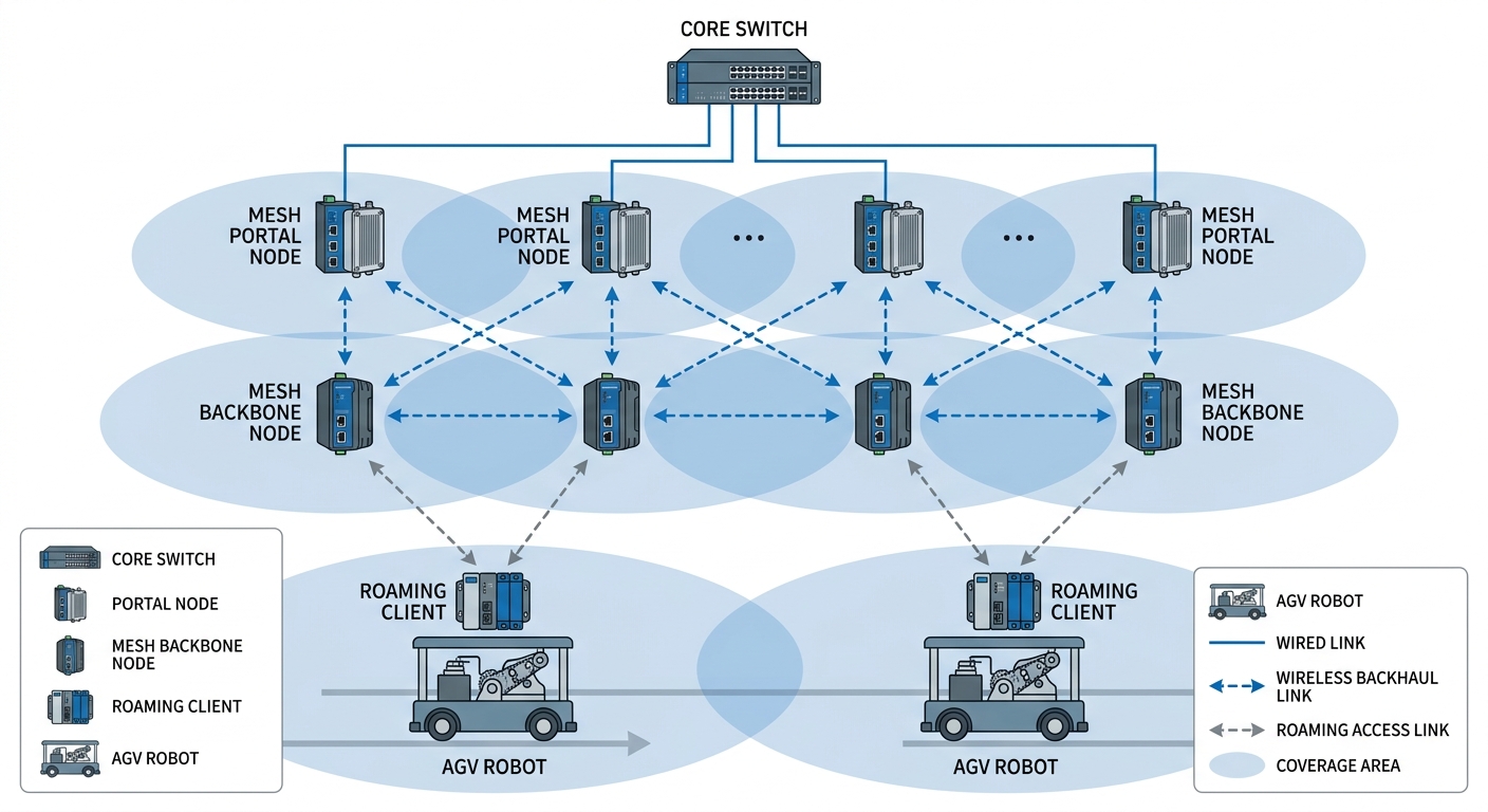
5.1 Model 1: Mesh as the Wireless Backbone, Robots as Clients (Recommended)
This is the most direct and most common approach. Mesh devices build the wireless coverage fabric, and robots roam across it as clients.
5.1.1 Model 1 Architecture: Mesh Backbone with Robot Clients
5.2 Model 2: Mesh Nodes as Mobile Access Points Travelling with the Robot (Unusual but Effective)
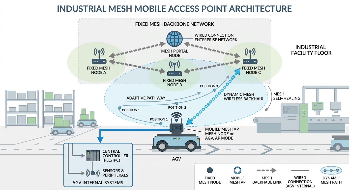
If some of your Mesh devices support wide-range power input and vibration-resistant design, a robot can carry a Mesh device configured in AP mode. This “mobile AP” links back to the fixed Mesh backbone over a wireless Mesh path while providing local Wi-Fi or Ethernet access for the robot’s own wired equipment (industrial PC, sensors).
In effect, this converts the “client roaming” problem into a “Mesh node mobility and topology self-healing” problem, leaving mobility to the Mesh protocol itself. It suits scenarios with special requirements on the client form factor.
5.2.1 Model 2 Architecture: Mesh Nodes as Mobile Access Points
6. Implementation Pitfalls: Three Engineering Details That Catch People Out
6.1 Confirm That the Mesh Equipment Really Supports Mobility
Not every industrial Mesh product is designed for mobile use. Many static Mesh nodes only extend coverage and have no handover logic optimized for mobile clients. Before purchasing, confirm:
- Whether the datasheet explicitly supports fast roaming (802.11k/v/r or a vendor-specific zero-switch technology)
- Whether the handover latency figures match your application — AGV scheduling typically requires below 100 ms, while precision control may need below 50 ms or even zero packet loss
6.2 Protocol Alignment Between Client and Mesh
If the Mesh nodes use a vendor-proprietary fast roaming protocol, the robot clients should ideally come from the same vendor or be verified compatible. Otherwise the link may fall back to standard 802.11 roaming, with degraded performance.
6.3 Robot Count and Roaming Domain Planning
Watch the upper limit on clients roaming simultaneously under a single AP/Mesh node. In logistics and warehousing with mobile forklifts, experience suggests no more than 16 mobile clients roaming per AP; in automated plants such as BYD, if a single AP must serve more than 20 AGVs or forklifts, node density must be increased with two to three layers of coverage. If you have many robots, you need to:
- Increase node density to reduce the load per coverage area
- Choose equipment models with higher client capacity
- Plan roaming domain boundaries so clients do not switch repeatedly between domains
6.4 Mesh Node Spacing: Recommended Distances and the Effect of Attenuation
Recommended Spacing by Scenario
| Deployment scenario | Obstruction / interference | Recommended node spacing | Mounting height |
|---|---|---|---|
| Indoor workshop / warehouse | Heavy obstruction from steel structures, racking and machinery | 30–80 m | 3–5 m, clear of metal columns |
| Underground roadway / tunnel | Multipath reflections, confined space | 80–120 m | Ceiling-mounted or side-wall mounted |
| Semi-outdoor plant yard / open stockyard | Intermittent obstruction by vehicles and stockpiles | 100–150 m | 5–8 m |
| Open area, elevated, unobstructed | Clear line of sight | 200–500 m | Above 8 m, maintaining line of sight |
| Extreme point-to-point (not recommended for routine use) | Pure line of sight, no multipath | ≤ 3000 m | High-elevation head-on alignment |
What Longer Distances Do: Quantitative Data from the Friis Equation
Node spacing is fundamentally a link budget problem. Using the measured parameters of the YN700B (5.8 GHz, 30 dBm transmit power, -97 dBm receiver sensitivity, 2×2 MIMO), the received power and link margin at each distance can be calculated with the Friis free-space transmission equation:
| Node spacing | Free-space path loss | Received power Pr | Link margin (relative to -97 dBm sensitivity) |
Signal assessment |
|---|---|---|---|---|
| 50 m | 81.7 dB | -51.7 dBm | 45.3 dB | Very strong, ample margin |
| 100 m | 87.7 dB | -57.7 dBm | 39.3 dB | Strong; upper limit of recommended indoor spacing |
| 200 m | 93.7 dB | -63.7 dBm | 33.3 dB | Good; recommended for semi-outdoor |
| 500 m | 101.7 dB | -71.7 dBm | 25.3 dB | Usable; upper limit for open areas |
| 1000 m (1 km) | 107.7 dB | -77.7 dBm | 19.3 dB | Fair; elevation required to maintain line of sight |
| 3000 m (3 km) | 117.3 dB | -87.3 dBm | 9.7 dB | Weak; insufficient margin, not recommended |
| 5000 m (5 km) | 121.7 dB | -91.7 dBm | 5.3 dB | Near the sensitivity limit; packet loss with the slightest interference |
| 8000 m (8 km) | 125.8 dB | -95.8 dBm | 1.2 dB | Virtually no margin; the datasheet maximum, achievable only under laboratory conditions |
Basis of calculation: free-space path loss L = 20·log₁₀(d) + 20·log₁₀(f) + 32.44, where d is distance in km and f is frequency in MHz (5800). Received power Pr = transmit power (30 dBm, conducted, excluding antenna gain) − L. Link margin = Pr − receiver sensitivity (-97 dBm). Real deployments incur a further 10–30 dB of loss from obstruction, multipath and interference; with 6 dBi directional antennas, roughly 6 dB can be added at each end.
Three Practical Consequences of Excessive Distance
- Packet loss rises steeply. When link margin falls below 10 dB (roughly beyond 3 km), any vehicle obstruction, metal reflection or co-channel interference can push received power below the -97 dBm sensitivity threshold, causing instantaneous loss. Industrial control has zero tolerance for loss — one lost packet can mean an emergency stop.
- Throughput roughly halves with each hop. Mesh traffic must traverse multiple relay hops to reach the Portal node. The YN700B delivers up to 96 Mbps in practice, and each hop typically costs 40–50% of throughput:
- 1 hop (direct to Portal): ~96 Mbps
- 2 hops: ~48 Mbps
- 3 hops: ~24 Mbps
- 5 hops: ~6 Mbps
- 10 hops (datasheet relay limit): ~1 Mbps, sufficient only for basic control signalling
- Roaming performance degrades. The wider the node spacing, the shorter the time window an AGV has to cross the coverage boundary — yet the signal at that boundary is weaker. The client spends longer in the weak-signal region, making sticky behaviour or failed handovers more likely. The overlap zone also shrinks, so the client may be forced into a hard switch before Make-before-break can complete.
Sources
- Zukaka YN700B datasheet: 5.8 GHz band, 30 dBm transmit power, -97 dBm receiver sensitivity (@20 MHz), 2×2 MIMO, 3–8 km range when elevated and unobstructed, up to 96 Mbps actual wireless throughput, Mesh scale ≥50 nodes, relay ≥10 hops
- Friis transmission equation: the fundamental radio propagation formula relating transmit power, distance, frequency and received power under ideal line-of-sight conditions
- Industrial wireless Mesh multi-hop throughput rule of thumb: general 802.11 Mesh engineering experience — single-radio Mesh loses roughly 40–50% of throughput per hop because transmit and receive share the channel in half-duplex operation
7. Application Scenarios and Selection Recommendations
7.1 Where Mesh Self-Organizing Networks Fit Best
- Cabling is difficult or too costly: underground roadways, mining panels, temporary work areas, retrofit of older plants
- Fast deployment and self-healing are required: frequent production line changes, or environments where equipment and vehicles obstruct links
- Coverage is mainly static or low-speed: inspection data backhaul, fixed equipment connectivity, video surveillance backhaul — insensitive to handover interruption
7.2 Where Dedicated Roaming Clients Fit Best
- High-speed or continuously moving automated equipment: AGV/AMR, RGV shuttle carts, stacker cranes, autonomous mining trucks
- Control commands that cannot be interrupted: robot motion control, safety obstacle-avoidance signals, remote operation
- Hard latency targets for handover: below 100 ms, or even below 10 ms with zero packet loss
7.3 Selection Cheat Sheet
| Your requirement | Focus on | Selection criteria |
|---|---|---|
| Many robots, frequent movement, tight real-time control | Roaming client performance | Handover latency (below 50 ms preferred), zero packet loss support, protocol compatibility with the Mesh nodes |
| Cabling is impractical on site, nodes may be added or removed temporarily | Mesh self-organization and self-healing | Network convergence time, throughput degradation after multiple hops, dual-band backhaul support |
| Robots have both Ethernet and serial devices | Client interface capability | Number and speed of Ethernet ports, serial type (RS232/485), Modbus gateway support |
| Dust, vibration, wide temperature swings | Industrial protection rating | Operating temperature range (-40 to 75 °C is typical industrial grade), ingress protection (IP40 or better), mounting method |
7.4 Specific Recommendations
Start by confirming the roaming specifications of your existing Mesh equipment:
- If the Mesh already supports fast roaming (802.11r or a vendor solution) → choose an industrial client that is compatible and whose handover figures meet your control cycle
- If the Mesh only provides basic coverage with weak roaming → use a high-performance industrial client on the robot side and increase Mesh node density to shrink each coverage area, compensating for the network side
7.5 The Built-In Advantage of Same-Vendor Pairing
The concept of “protocol alignment” mentioned earlier is easiest to understand with the Zukaka combination:
- Identical RF parameters, seamless signal boundaries. The YN700B Mesh node and the YN300B roaming client both use 5.8 GHz, 30 dBm transmit power, -97 dBm receiver sensitivity and 2×2 MIMO — so the client’s roaming scans and the AP’s beacons operate on the same RF baseline. You will not see “the AP covers the area but the client cannot hear it”, or the reverse.
- Common protocol stack, handover suggestions acted on reliably. Roaming trigger thresholds, channel priorities and key derivation parameters sent by the Mesh node are executed by the client without translation. Across vendors these steps often need three to five minutes of compatibility verification; a same-vendor solution works out of the box.
- Consistent power and thermal strategy. The two share overlapping supply ranges (7–48 V / 12–48 V), so one power plan covers both; both are rated -40 °C to +65 °C, so the same industrial protection approach applies.
- Predictable scale and coverage. The YN700B supports ≥50 Mesh nodes and ≥10 relay hops. With YN300B clients attached, the network ceiling is the Mesh backbone’s ceiling — no mismatch such as “the Mesh supports 50 nodes but the clients cap out at 30”.
References
- IEEE 802.11k-2011: Amendment 2: Radio Resource Management Enhancements
- IEEE 802.11r-2008: Amendment 3: Fast BSS Transition
- IEEE 802.11v-2011: Amendment 8: Wireless Network Management
- BYD FinDreams Technology plant AGV wireless roaming deployment case (public technical presentation)
- MIIT Announcement No. 52 of 2019, Catalogue and Technical Requirements for Micro-power Short-range Radio Transmission Equipment (domestic 5.8 GHz band, EIRP ≤ 33 dBm)
- FCC 47 CFR Part 15.247 (United States, 5725–5850 MHz power limits)
- ETSI EN 301 893 (harmonized standard for 5 GHz wireless access equipment in the European Union)
Frequently Asked Questions
Q: I already have Mesh equipment. Do I still need to buy separate roaming clients?
It depends on how much communication interruption your application can tolerate. For inspection video backhaul or non-real-time monitoring, where an occasional stutter is acceptable, built-in Mesh roaming is sufficient and no extra spend is needed. For AGV/AMR control or remote mining-truck operation, where a single break is an incident, the client-side decision authority and break-before-make logic of built-in Mesh roaming are not enough — dedicated industrial roaming clients are required.
Q: Must dedicated roaming devices come from the same vendor as the Mesh?
Not necessarily, but it is strongly recommended. Standard 802.11k/v/r should in theory interoperate across vendors, but in practice compatibility of vendor-proprietary fast roaming protocols varies widely. If the client and the Mesh come from different vendors, steps such as the 802.11r fast handshake and key derivation may fail, degrading performance to that of ordinary roaming. The best practice is to verify compatibility in advance.
Q: How much does a dedicated roaming client cost, and what if the budget is limited?
Industrial vehicle-mounted clients range from a few hundred to several thousand yuan, depending on performance grade, interface type and ingress protection. If the budget is tight, take two steps first: confirm whether your Mesh equipment already supports 802.11r, which can save part of the extra spend; and increase Mesh node density to shrink each coverage area, reducing how often clients need to hand over and lowering the performance demanded of them.
Q: How many Mesh nodes and robots count as a “large” deployment?
Client capacity varies by device, but a general rule of thumb is no more than 16–32 clients roaming simultaneously under a single AP/Mesh node. If your robot count exceeds that, you need higher Mesh node density, well-planned roaming domain boundaries, or an enterprise-grade Mesh solution with greater client capacity. The larger the deployment, the more important roaming domain planning and channel isolation become.
In specific industries: for mobile forklifts in logistics and warehousing, experience suggests no more than 16 per AP; in automated plants such as BYD, if a single AP must serve more than 20 AGVs, node density must be increased with two to three layers of coverage.
Q: Is “zero packet loss” at the handover instant real?
For dedicated roaming devices built on a Make-before-break architecture, zero packet loss is a committed, measurable figure — traffic is switched seamlessly from an already-established standby path, with no break in the link. But it depends on two preconditions: the Mesh backbone itself must be stable, and the client and Mesh nodes must be fully aligned on the roaming protocol. If either precondition fails, “zero packet loss” is just marketing.
Procurement FAQs (common buyer questions, answered by the supplier)
Q: Must Mesh equipment and roaming clients be purchased together? Can procurement be phased?
Phased procurement is entirely feasible, and we recommend it. It lowers the initial outlay and lets you validate results with real traffic data in phase one before deciding whether — and how many — clients to add in phase two.
Our solution supports phasing without rework:
- Phase one, Mesh backbone only: the YN700B Mesh board already includes baseline roaming (802.11k/v/r support), so buying only Mesh nodes first still delivers coverage and basic roaming — nothing is wasted.
- Phase two, clients as needed: once robot numbers grow and deterministic handover becomes a requirement, add one YN300B roaming client per robot. Because Mesh and clients share the same vendor and protocol, they are plug-and-play later — no re-networking or backbone changes.
- We plan headroom for mobility from phase one: for example, sizing at ≥16 clients per AP and ≥50 nodes for network scale, so you do not have to rework later because the initial sizing was too conservative.
In short: build the network first, add endpoints later. Spend is phased, risk is contained, and we support you through both phases.
Q: Is the equipment compliant? What certifications and documentation are needed for domestic sales and acceptance?
Compliance is a precondition of shipment — you can rely on that.
Our devices are configured for compliance by destination market before dispatch, and we can supply full documentation at purchase:
- SRRC type approval certificate — domestic 5725–5850 MHz band, EIRP held within the ≤33 dBm limit, with the certificate model matching the purchased model exactly, never substituted
- Third-party RF test report — transmit power, frequency range, spurious emissions and other parameters all within limits
- ISO 9001 quality management certification — ensuring production consistency
- Export projects: regional certification versions are available, such as FCC ID for the United States, CE for the European Union (including ETSI EN 301 893 test reports) and TEC/TELEC conformity for Japan
Q: Can we start with a small trial batch? How would you support validation?
We very much welcome a POC with sample units before volume purchase. We understand the risk of committing to volume in industrial projects and prefer to let measured data speak rather than just handing you a datasheet.
What we can provide:
- A minimum validation kit: two YN700B Mesh nodes plus one YN300B roaming client, with support for deploying them in your real work area
- A standardized test plan and tools: a concrete test script — run the real route continuously for at least 2 hours, crossing node boundaries at least 3–5 times, with continuous ping / iperf traffic at one end, recording packet loss count, maximum outage duration and latency jitter quantitatively
- Engineer support on site or remotely: tuning roaming threshold parameters and channel planning so you measure our solution at its best, not at its worst after trial and error
- A formal test report: results confirmed jointly by you and us, usable as the basis for volume purchase and acceptance
Our commitment on results: for general control applications, no more than 2 packets lost per handover and a maximum outage of 50 ms; for precision control or safety applications, zero packet loss and a maximum outage below 10 ms. If measured results fall short, we help optimize or accept a return — you do not carry the cost of validation.
Q: What are the minimum order quantity and lead time?
We set no hard threshold on order size and support everything from samples to volume:
- MOQ: 1–2 units can be ordered at the sample stage; price breaks apply from 100 units
- Lead time: standard stock items usually ship within 3–7 working days; projects requiring custom power levels, bands, interfaces or enclosures typically take 2–4 weeks
Q: How should total cost of ownership (TCO) be calculated? Will expansion and maintenance be expensive later?
Long-term cost of ownership was designed in from the start — we are not just selling a box:
- Smooth expansion, no rebuild: the YN700B supports ≥50 nodes and ≥10 relay hops. When you add a production line, simply add nodes and the network converges automatically — no rip-and-replace. If you outgrow that ceiling, we offer higher-capacity options for a smooth upgrade.
- Low-touch maintenance with remote bulk operations: devices support remote web configuration and bulk firmware upgrades. Adjusting roaming thresholds, changing power or upgrading firmware needs no site visit, keeping long-term labour costs low.
- Controllable spares: we recommend stocking 10–15% of purchase volume. The YN300B vehicle-mounted client is built to industrial standards (-40 to +65 °C, wide-range power input, vibration-resistant design), keeping failure rates low; if a unit does fail, we provide fast replacement support.
We can work through the TCO with you: equipment cost, spares, expansion and maintenance labour taken together. The extra spend on dedicated roaming clients typically pays for itself within six to twelve months by avoiding a single handover-related failure. If helpful, our engineers can produce a calculation tailored to your site.
Q: How can I confirm this is genuinely dedicated roaming and not a rebadged ordinary AP?
That concern is entirely reasonable, and we would rather you verify with measured figures than take our word for it. We proactively offer three verifiable pieces of evidence:
- Concrete measured handover latency, not adjectives: the YN300B roaming client achieves measured handover latency below 10 ms with zero packet loss — you can measure this yourself during the POC. We do not shy away from quantification.
- Dual-radio architecture, scanning does not occupy the service channel: the YN300B uses a dual-radio design, with one radio dedicated to the active session and the other scanning independently in the background. Verification is simple: run continuous traffic on an AGV while it crosses a coverage boundary — you will see the traffic stream stay up and throughput stay flat. An ordinary single-radio AP will always steal service bandwidth while scanning, which becomes obvious the moment it is installed.
- Make-before-break logic: our handover establishes a parallel connection to the new node over the secondary radio while the original link is still healthy, and traffic switches seamlessly from the hot-standby path — that is how zero packet loss is achieved. A device that merely claims “802.11r support” is break-before-make, which is fundamentally different.